Comparison of bootstrapping approaches for identifying variance of predictive performance
Background
Bootstrapping is a helpful technique for identifying the variance of an estimate in a given sample when no other data are available. In the case of the evaluation of clinical prediction models, bootstrapping can be used to estimate confidence intervals around performance metrics such as the Brier score, the c-statistic, and others. When the original model and its tuning parameters, and the original dataset are available, the data can be resampled and the model refit on each replicate to make predictions. These predictions can then be used to calculate a performance metric. However, sometimes only the predicted probabilities of the original model on the original dataset are available. In this case, the predicted probabilities can be resampled and the performance metric can be calculated on each of these replicates. How do these approaches compare?
Build a model
Similar to the model built in another blog post about the Brier Score, let’s build a model with the abalone dataset.
# set seed
set.seed(24601)

# load libraries for plotting
library(ggplot2)

# get data
df <- read.csv('https://archive.ics.uci.edu/ml/machine-learning-databases/abalone/abalone.data')
names(df) <- c('sex', 'length', 'diameter', 'height', 'weight_whole',
               'weight_shucked', 'weight_viscera', 'weight_shell', 'rings')
# inspect data
knitr::kable(head(df))| sex | length | diameter | height | weight_whole | weight_shucked | weight_viscera | weight_shell | rings |
|---|---|---|---|---|---|---|---|---|
| M | 0.350 | 0.265 | 0.090 | 0.2255 | 0.0995 | 0.0485 | 0.070 | 7 |
| F | 0.530 | 0.420 | 0.135 | 0.6770 | 0.2565 | 0.1415 | 0.210 | 9 |
| M | 0.440 | 0.365 | 0.125 | 0.5160 | 0.2155 | 0.1140 | 0.155 | 10 |
| I | 0.330 | 0.255 | 0.080 | 0.2050 | 0.0895 | 0.0395 | 0.055 | 7 |
| I | 0.425 | 0.300 | 0.095 | 0.3515 | 0.1410 | 0.0775 | 0.120 | 8 |
| F | 0.530 | 0.415 | 0.150 | 0.7775 | 0.2370 | 0.1415 | 0.330 | 20 |
# Let's predict whether or not an abalone will have > 10 rings
m <- glm(I(rings > 10) ~ ., data = df, family = binomial)
preds_m <- predict(m, type = 'response')
Performance metric
Let’s calculate the Brier score as a measure of model performance.
brier_score <- function(preds, obs) {
  mean((obs - preds)^2)
}
Boostrapping the predicted probabilities only
Now let’s estimate the 95% confidence interval of the Brier score using only the predicted probabilities.
N <- 1000

get_boot_est_preds <- function(preds, obs, metric) {
  idx <- sample(length(preds), replace = TRUE)
  metric(preds[idx], obs[idx])
}

reps_pred <- replicate(N, get_boot_est_preds(preds_m, df$rings > 10, brier_score))
Bootstrapping to refit the model on each replicate
get_boot_est_mod <- function(df, metric) {
    idx <- sample(nrow(df), replace = TRUE)
    m_b <- glm(I(rings > 10) ~ ., data = df[idx,], family = binomial)
    preds_m_b <- predict(m_b, type = 'response')
    metric(preds_m_b, df[idx,]$rings > 10)
}

reps_model <- replicate(N, get_boot_est_mod(df, brier_score))
Optimism corrected bootstrapping to refit the model on each replicate
As pointed out by Ewout Steyerberg, these estimates should be optimism-corrected for potential overfitting. Let’s look at the difference in estimates if we make predictions on the initial dataset rather than on the bootstrapped sample.
get_boot_est_mod <- function(df, metric) {
    idx <- sample(nrow(df), replace = TRUE)
    m_b <- glm(I(rings > 10) ~ ., data = df[idx,], family = binomial)
    preds_m_b <- predict(m_b, data = df, type = 'response')
    metric(preds_m_b, df$rings > 10)
}

reps_model_opt <- replicate(N, get_boot_est_mod(df, brier_score))
Evaluate results
Let’s look at the distrbution of the Brier score estimates using both approaches.
res <- rbind(data.frame(brier_score = reps_pred,
                        approach = 'predictions'),
             data.frame(brier_score = reps_model,
                        approach = 'refit_model'),
             data.frame(brier_score = reps_model_opt,
                        approach = 'refit_opt'))

# Plot distribution of bootstrapped Brier scores
ggplot(res, aes(brier_score, color = approach)) +
  geom_density() +
  theme_bw()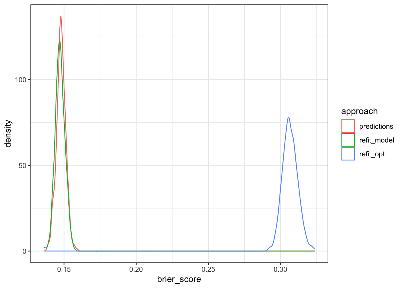
We can calculate 95% confidence intervals using a simple percentile approach.
calc_ci_95 <- function(v) {
  q <- format(quantile(v, probs = c(0.025, 0.975)), digits = 5)
  paste0('(',q[1],' to ',q[2],')')
  }

cat('CI using bootstrapped estimates from predictions only:',
    calc_ci_95(reps_pred),'\n')
## CI using bootstrapped estimates from predictions only: (0.14153 to 0.15414)cat('CI using bootstrapped estimates from refitting the model:',
calc_ci_95(reps_model),'\n')## CI using bootstrapped estimates from refitting the model: (0.14128 to 0.15395)cat('CI using bootstrapped estimates from refitting the model with an optimism correction:',
calc_ci_95(reps_model_opt),'\n')## CI using bootstrapped estimates from refitting the model with an optimism correction: (0.29691 to 0.31728)Summary
While not exactly the same, the first two approaches yield very similar results. However, this outcome may vary depending on potential bias in the original dataset, and the sensitivity of the model to such bias. The third approach demonstrates the likely high degree of overfitting in this model, and the need to properly correct for optimism when reporting predictive performance in the absence of a separate testing sample.
Assistant Professor of Medicine and Informatics
I am a pulmonary and critical care physician at the University of Pennsylvania Perelman School of Medicine, and core faculty member at the Palliative and Advanced Illness Research (PAIR) Center. My work seeks to translate innovations in artificial intelligence methods into bedside clinical decision support systems that alleviate uncertainty in critical clinical decisions. My research interests include clinical informatics, artificial intelligence, natural language processing, machine learning, population health, and pragmatic trials.