Transportation data in R: Why yes, yes you can

Not infrequently I am in a research meeting and someone says, “It would be really cool to get data on travel times for people. But I don’t know where to find that.” Here you will find just that. Please note that Google Maps terms of service are relevant for large data requests and potential privacy concerns for protected health information.

Case

Mr. Jones spends all his time at a coffee shop. Mr. Jones has hypertension, diabetes, and hyperlipidemia, and it doesn’t seem likely he will visit his primary care doctor anytime soon. Can we describe his potential travel time between his favorite coffee shop and his primary care doctor to better understand his transportation barriers? Why yes, yes we can.

Transport

library(ggmap)
# quick start to ggmap: https://github.com/dkahle/ggmap

# Specify where Mr. Jones is and where he's going
# you can also use specific addresses if you already have them
origin <- 'Hobbs Coffee Shop, Swarthmore'
destination <- 'Penn Center for Primary Care, Philadelphia'

# get some routes -- driving
my_commute_drive <- route(origin, destination, 
    structure = 'route', mode = 'driving')
print(my_commute_drive)

      m    km     miles seconds   minutes       hours leg       lon      lat
1    30 0.030 0.0186420       8 0.1333333 0.002222222   1 -75.35005 39.90210
2   162 0.162 0.1006668      56 0.9333333 0.015555556   2 -75.35033 39.90226
3  1047 1.047 0.6506058     123 2.0500000 0.034166667   3 -75.35089 39.90116
4  1829 1.829 1.1365406     214 3.5666667 0.059444444   4 -75.35296 39.89203
5   747 0.747 0.4641858      63 1.0500000 0.017500000   5 -75.34469 39.87802
6  4516 4.516 2.8062424     190 3.1666667 0.052777778   6 -75.35102 39.87342
7  5664 5.664 3.5196096     189 3.1500000 0.052500000   7 -75.30839 39.86862
8  5534 5.534 3.4388276     247 4.1166667 0.068611111   8 -75.24609 39.88126
9  2236 2.236 1.3894504     126 2.1000000 0.035000000   9 -75.19435 39.90546
10 1111 1.111 0.6903754      49 0.8166667 0.013611111  10 -75.19280 39.92460
11  347 0.347 0.2156258      20 0.3333333 0.005555556  11 -75.20004 39.93279
12  907 0.907 0.5636098     145 2.4166667 0.040277778  12 -75.19939 39.93587
13 1556 1.556 0.9668984     344 5.7333333 0.095555556  13 -75.19639 39.94367
14  141 0.141 0.0876174      31 0.5166667 0.008611111  14 -75.19798 39.95667
15  114 0.114 0.0708396      30 0.5000000 0.008333333  15 -75.19761 39.95791
16  105 0.105 0.0652470      41 0.6833333 0.011388889  16 -75.19893 39.95809
17   NA    NA        NA      NA        NA          NA  NA -75.19930 39.95843

Or try public transit.

# route -- transit
my_commute_transit <- route(origin, destination, 
    structure = 'route', mode = 'transit')
print(my_commute_transit)

      m     km      miles seconds   minutes      hours leg       lon      lat
1    49  0.049  0.0304486      39  0.650000 0.01083333   1 -75.35005 39.90210
2 16750 16.750 10.4084500    1560 26.000000 0.43333333   2 -75.35083 39.90222
3   239  0.239  0.1485146     239  3.983333 0.06638889   3 -75.18166 39.95667
4  1624  1.624  1.0091536     180  3.000000 0.05000000   4 -75.18325 39.95489
5   424  0.424  0.2634736     313  5.216667 0.08694444   5 -75.20197 39.95719
6    NA     NA         NA      NA        NA         NA  NA -75.19930 39.95843

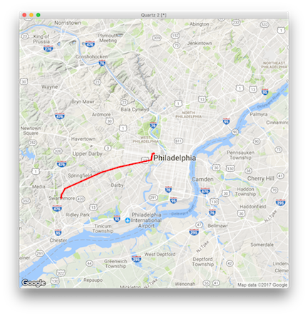
Let’s see what a walk would look like.

# route -- walking
my_commute_walk <- route(origin, destination, 
    structure = 'route', mode = 'walking')
print(my_commute_walk)

# now plot the commute path
qmap(destination, zoom = 11) + 
    geom_path(aes(x=lon, y = lat), color = 'red', 
        size = 1.5, data = my_commute_walk, 
        lineend = 'round')

Mr. Jones, inspired by this map, just put down his triple-shot latte and is walking to his doctor’s office right now.